Rate Is Not Capacity: What a Pressure Ceiling Does to a Storage Ranking

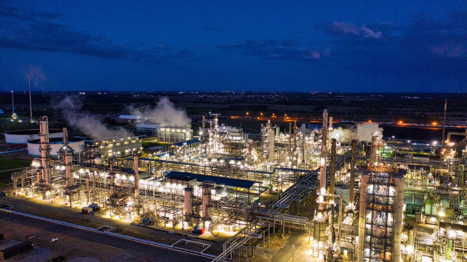
Every public number attached to a working CO2 storage project is a rate. Northern Lights, owned by Equinor, Shell and TotalEnergies, describes an initial capacity of 1.5 million tonnes per year expanding to a minimum of 5 million tonnes, injected into a storage complex named Aurora that sits 2,600 metres under the seabed of the North Sea [1]. ExxonMobil's Baytown announcement of 1 March 2022 says the carbon capture infrastructure for the project would have the capacity to transport and store up to 10 million metric tons of CO2 per year [2]. ADNOC took a final investment decision on the Habshan project on 6 September 2023 with the capacity to capture and permanently store 1.5 million tonnes per annum, which the same release says will triple ADNOC's carbon capture capacity to 2.3 mtpa [3]; a month later the company put a second 1.5 mtpa project on top of that and stated a target it had doubled to 10 mtpa of CO2 by 2030 [4].

Tonnes per year. Every one of them.

Now read the Northern Lights page again for what it does not contain. It gives the owners, the reservoir name, the injection depth and two rates, and it never states how much CO2 the Aurora complex holds in total [1]. That absence is the honest position. A rate is a commitment about wells and compressors. A total is a claim about rock, and the number that governs it is not the one most screening tools compute.

A rate held for a project lifetime is a cumulative mass

Held for 25 years, 1.5 million tonnes a year is 37.5 million tonnes. At 5 million a year it is 125 million. At 10 million a year it is 250 million. Those are the masses the rock has to accept, and the question a site-screening model is really being asked is which candidate accepts the largest one.

There are two formulas in circulation for answering it, and they are not the same formula wearing different notation.

The volumetric formula, and the one that replaces it in a closed system

IEAGHG Technical Report 2023-05 sets both out side by side. The open-system case is a volume balance: replace brine with CO2 inside the pore volume, discount for irreducible water, and you have the theoretical volume [6]. Written as a mass, the same report quotes the US Department of Energy form,

$$G_{\mathrm{CO_2}} \;=\; A \, h_n \, \varphi_c \, (1 - S_w) \, \rho_{\mathrm{CO_2}} \, E$$

FormulaLaTeX

Copy LaTeX

where E is the storage efficiency factor [6]. NETL's own CO2-SCREEN manual writes the saline case as a product of the gross geometry and a single efficiency term,

$$G_{\mathrm{CO_2}} \;=\; A_t \, h_g \, \varphi_{tot} \, \rho_{\mathrm{CO_2}} \, E_{saline}, \qquad E_{saline} \;=\; E_A \, E_h \, E_\varphi \, E_V \, E_d$$

FormulaLaTeX

Copy LaTeX

with E_saline defined as the fraction of the total pore volume that is filled by CO2, and the five terms auto-populated from lithology and depositional environment [7]. That is the formula behind a national storage atlas, and it is the formula a screening feature vector is built to feed: area, thickness, porosity, net-to-gross, depth, lithology.

The closed-system case is a different balance. When the boundary restricts lateral flow, the injected volume is accommodated by compressing the pore and fluid system rather than by pushing brine away, and the same report gives it as its Equation 2 [6]:

$$V_{\mathrm{CO_2}} \;=\; V \, \phi \, (c_w + c_p) \, \Delta p$$

FormulaLaTeX

Copy LaTeX

with c_w and c_p the water and rock compressibilities and Delta p the allowable pressure increase within the geomechanical limits of the reservoir and caprock [6].

Divide both sides by the pore volume V phi. The storage efficiency of a closed aquifer is

$$E_p \;=\; c_t \, \Delta p$$

FormulaLaTeX

Copy LaTeX

and nothing else. Not porosity. Not net-to-gross. Not thickness. Total compressibility times allowable pressure rise.

The arithmetic first, because it is the easy half

Put a plausible total compressibility of 10^{-4} per bar and an allowable rise of 50 bar into that expression and the pressure-limited storage efficiency is 0.5% of pore volume. That number is our derivation from the sourced formula, not a figure either source prints; what the sources supply is the formula and the comparison set.

The comparison set is unflattering. For bulk-volume calculation of regional aquifer formations the IEAGHG report says a storage efficiency factor of 2% is suggested, based on work by the US DOE, and cites Frailey's Monte Carlo simulations giving P50 storage efficiencies between 1.8% and 2.2% of the bulk volume, with low and high values of 1% and 4% [6]. Those are efficiencies of the bulk volume, and the 0.5% above is of pore volume, so the two cannot be divided into one another; a bulk-volume factor is the smaller number for the same rock, by roughly the porosity times the net-to-gross. Later on the same page, reviewing the Norwegian storage atlas, the report states the two regimes without switching basis: storage efficiencies used in closed systems are generally less than 1% and more than this in open or partially open systems, where up to 20% is used [6]. That is a description of atlas practice rather than a general rule, and the efficiency it reports is defined against accessible pore volume, which is the basis the 0.5% above is on. The derived figure sits inside its closed-system band. The volumetric atlases ship the open-system numbers.

This is the part of the argument Thibeau and Mucha published in 2011. Working at TOTAL SA in Pau and at MATMECA in Talence, they separated two pressure effects during injection: the local overpressure around an injector, which more injectors can address, and the regional-scale pressure increase in closed or low-permeability formations, which they cannot. Their recommendation was explicit, that a screening study ranking aquifers should evaluate CO2 storage capacities using a pressure and compressibility formula rather than a volumetric approach, and their illustrative case was the Utsira aquifer in the North Sea [5]. The volumetric approach is what the public atlases still ship 15 years later, and it is what a model trained on atlas labels learns.

The half that is not arithmetic

An efficiency factor read off the wrong system is a scaling error. A team that knows about it applies a haircut and moves on. What survives the haircut is the ordering, and the ordering is where the damage sits, because a screening tool is not usually asked for a number. It is asked which site to characterise first.

Look at the two expressions again. Volumetric capacity is linear in porosity and net-to-gross and carries a common efficiency factor. Pressure-limited capacity is linear in total compressibility and in the allowable pressure rise. Porosity and compressibility are different rock properties and they are not proportional to one another across rock types, so the two expressions do not have to agree about which candidate is largest. Whether they agree is set by how open the boundary is, and the boundary condition is a basin-scale property, not a column in a well header.

The exhibit below makes that concrete. Three schematic candidate stores, each with its own bulk volume, porosity, net-to-gross, compressibility multiple and boundary conductance, ranked twice.

boundary openness assumed: 0.20 (0 closed to 1 open)allowable pressure rise: 50.0 bar (10 to 120)reference total compressibility: 1.00e-4 per bar (3e-5 to 3e-4, log)volumetric efficiency factor: 2.00% (0.5 to 4)

The partially open case is the volume balance carried one step further. If a fraction a of the injected volume leaves across the boundary instead of being taken up by compression, then only the remaining (1-a) has to be absorbed by the pore and fluid system, so

$$(1-a)\,V_{inj} \;=\; V \phi \, c_t \, \Delta p \qquad \Longrightarrow \qquad V_{inj} \;=\; \frac{V \phi \, c_t \, \Delta p}{1-a}$$

FormulaLaTeX

Copy LaTeX

At a = 0 that is Equation 2 exactly. A screening study assumes one openness for a whole play; each candidate converts that assumption into its own relief fraction through its own boundary conductance, which is what the exhibit's openness control does.

Three things follow, and the exhibit is where you check them rather than take them.

The first is that the volumetric ranking never moves. The efficiency factor is common to all three candidates, so it scales every volumetric capacity by the same amount and cancels out of every comparison. Whatever value the atlas assigns, the volumetric ranking is the pore-volume ranking.

The second is that the allowable pressure rise and the reference compressibility cannot move the pressure ranking either, for the same reason. They are common multipliers. Drag either of them from one end of its range to the other and every pressure-limited capacity changes, the ratio in the top right changes, and neither column re-orders. Exactly one control re-orders anything, and it is the boundary openness.

The third is the finding. The two rankings coincide only for openness between 0.311 and 0.447, which is 13.6% of that control's range, so they disagree over the other 86.4%, both ends included. The exhibit opens at 0.20, inside the disagreement, where the store holding 49% more pore volume than its nearest rival ranks last on pressure headroom. Drag the openness up and the amber flag goes out at 0.311 and comes back on at 0.447.

That the agreement region is a single window rather than a scatter of patches is not luck. For any two candidates the ratio of their pressure-limited capacities is

$$\frac{g_i}{g_j} \;=\; \frac{P_i}{P_j} \cdot \frac{1 - \alpha \kappa_j}{1 - \alpha \kappa_i}, \qquad \frac{d}{d\alpha}\!\left(\frac{1 - \alpha \kappa_j}{1 - \alpha \kappa_i}\right) \;=\; \frac{\kappa_i - \kappa_j}{(1 - \alpha \kappa_i)^2}$$

FormulaLaTeX

Copy LaTeX

whose sign is the constant sign of kappa_i - kappa_j. Each pair therefore crosses at most once, the agreement set is an intersection of half-intervals, and it is a single interval or empty. The disagreement region is its complement, which is why it cannot be a bubble in the middle.

What this does to a learned ranker

A screening model trained to predict storage capacity is trained on labels. The labels available at national scale are volumetric, because that is what the atlases compute, and the features available are the ones the volumetric formula wants, because that is what the atlases record. Both halves of the supervision come from the same formula.

Such a model can be excellent and still be pointed at the wrong quantity. Its residuals will be small against its own labels. Its held-out score will be reassuring, because the held-out sites were labelled the same way. And its top-ranked candidate will be whichever compartment holds the most pore space, which, on the exhibit's numbers, is the candidate the pressure ranking puts last at the boundary assumption the exhibit opens on, and puts first only once the boundary is assumed open enough for the two rankings to meet.

Two properties decide the pressure ranking and neither reliably appears in a screening feature vector. Total compressibility is one: pore compressibility is a mechanical property measured on core under stress, not a log-derived curve, and it does not follow from porosity in a way a model can regress. The other is worse. Boundary conductance is not a property of the candidate at all. It is a property of the compartment the candidate sits in, and the IEAGHG report is direct about it, that compartmentalisation plays a key role in the calculation of storage efficiency in saline aquifers and that where boundary conditions restrict lateral flow it is necessary to treat the domain as a closed system and calculate accordingly [6]. That is a structural interpretation, not a feature.

So the failure is not that the ranker is inaccurate. It is that the ranker is accurate about a quantity whose ordering flips on an input it was never given.

Our own loop ranks, which is why this is a working concern rather than a comment

We built a five-agent CCS screening loop that ingests well data, screens reservoir and caprock intervals, and ranks the survivors by a Darcy-simplified injectivity index, with automatic fallback re-routing when a primary interval fails caprock integrity. On a ten-well synthetic North Sea and Gulf Coast set it eliminated four candidates, ranked six, and ran in under two seconds [8]. We followed it with a crustal-scale version [9].

Both of those rank. That is the whole product. And a ranker is worth exactly as much as the constraint it encodes, which is why the constraint question is the one we ask first now. Injectivity is a rate constraint: it answers how fast a well can accept CO2 at a given pressure rise. Cumulative capacity is a different constraint with a different governor, and a loop that ranks on the first and is read as ranking on the second will hand a project a confident, auditable, well-formatted ordering of the wrong thing.

The auditability we were pleased about makes this sharper, not softer. A per-criterion audit trail records which threshold each candidate passed. It does not record that the threshold set omitted a governing constraint. Nothing in the trail will look wrong.

What to ask before a screening ranking sets the characterisation budget

Three questions, in order.

Which formula produced the labels this model was fitted on? If the answer is a national atlas, it is the volumetric one, and its efficiency factor is a P50 from a Monte Carlo over lithology and depositional environment rather than a property of the candidate [6][7].

What is the compartmentalisation interpretation for each candidate, and who signed it? Not the porosity, not the permeability. The lateral extent over which pressure will actually communicate during 25 years of injection. Where that interpretation does not exist, the pressure-limited number cannot be computed at all, and the honest output is a ranking with a stated boundary assumption attached rather than a ranking.

And what is the allowable pressure rise, from what geomechanical basis? It multiplies the pressure-limited capacity linearly and it is the only term in that expression an operator can influence after the rock is chosen.

None of this makes the volumetric formula wrong. It makes it a screen for a different question. The published rates from Northern Lights, Baytown and Habshan are rates because rates are what those projects have committed to and rates are what they can measure. The cumulative masses those rates imply belong to a different calculation, and the ordering that calculation produces is not the ordering a pore-volume model returns.

Key takeaways

1. 1Every public figure on the working projects is a rate. Northern Lights states 1.5 million tonnes a year rising to a minimum of 5 million, Baytown up to 10 million metric tons a year of transport and storage, Habshan 1.5 mtpa tripling ADNOC's installed capacity to 2.3 mtpa. The Northern Lights page states depth, owners and reservoir name and gives no total capacity for Aurora at all.
2. 2Divide the IEAGHG closed-system equation through by pore volume and the pressure-limited storage efficiency is total compressibility times allowable pressure rise, with no other term. At 1e-4 per bar and 50 bar that is 0.5% of pore volume, inside the under-1% band the same report reports for closed systems in the Norwegian atlas. The volumetric factors the atlases use are open-system numbers, where that report says up to 20% is used.
3. 3Thibeau of TOTAL and Mucha recommended in 2011 that screening studies rank aquifers with a pressure and compressibility formula rather than a volumetric one, separating local overpressure that more injectors can fix from regional pressure buildup in closed formations that they cannot.
4. 4The scaling error is the easy half. The volumetric formula is linear in porosity and the pressure formula is linear in compressibility, and the two are not proportional across rock types, so the formulas induce different orderings. In the exhibit the two rankings coincide only for boundary openness between 0.311 and 0.447, 13.6% of the range, and disagree over the other 86.4% including both ends.
5. 5Each pair of candidates crosses at most once, because the ratio of their pressure-limited capacities is monotone in the openness, so the agreement region is one interval rather than a scatter of patches. For these three candidates that interval sits strictly inside the range, which is what puts the disagreement at both extremes.
6. 6Neither of the two properties that decide the pressure ranking sits in a screening feature vector. Pore compressibility is measured on core under stress and does not follow from porosity; boundary conductance is a property of the compartment rather than of the candidate, and is a structural interpretation someone has to sign.
7. 7Our own five-agent CCS loop ranks candidates by a Darcy-simplified injectivity index, which is a rate constraint. Cumulative capacity has a different governor, and a per-criterion audit trail records which thresholds a candidate passed, never that the threshold set omitted a governing one.

References

[1] Northern Lights JV. What we do. https://norlights.com/what-we-do/

[2] ExxonMobil. ExxonMobil planning hydrogen production, carbon capture and storage at Baytown complex. 1 March 2022. https://corporate.exxonmobil.com/news/news-releases/2022/0301_exxonmobil-planning-hydrogen-production-carbon-capture-and-storage-at-baytown-complex

[3] ADNOC. ADNOC to Invest in One of the Largest Integrated Carbon Capture Projects in MENA. 6 September 2023. https://www.adnoc.ae/en/news-and-media/press-releases/2023/adnoc-to-invest-in-one-of-the-largest-integrated-carbon-capture-projects-in-mena

[4] ADNOC. ADNOC Takes FID on World's First Project That Aims to Operate with Net Zero Emissions. 5 October 2023. https://www.adnoc.ae/en/news-and-media/press-releases/2023/adnoc-takes-fid-on-worlds-first-project-that-aims-to-operate-with-net-zero-emissions

[5] Thibeau, S. and Mucha, V. Have We Overestimated Saline Aquifer CO2 Storage Capacities? Oil and Gas Science and Technology, vol. 66 no. 1, pp. 81 to 92, 2011. DOI 10.2516/ogst/2011004. https://inis.iaea.org/records/k99jw-4ef09

[6] IEAGHG. Classification of Total Storage Resources and Storage Coefficients. Technical Report 2023-05. https://publications.ieaghg.org/technicalreports/2023-05%20Classification%20of%20Total%20Storage%20Resources%20and%20Storage%20Coefficients.pdf

[7] National Energy Technology Laboratory. CO2 Storage prospeCtive Resource Estimation Excel aNalysis (CO2-SCREEN) User's Manual. https://netl.doe.gov/projects/files/CO2StorageprospeCtiveResourceEstimationExcelaNalysisCO2SCREENUsersManual_050820.pdf

[8] EarthScan. Agentic CCS: Months of Site Screening in Minutes. https://earthscan.io/insights/agentic-ccs-site-screening-five-agent-loop

[9] EarthScan. Agentic CCS Crustal Screening: Months to Minutes. https://earthscan.io/insights/agentic-ccs-crustal-screening-months-to-minutes