Automated FMI-log correlation via unsupervised CNN segmentation

“
The pitch is not subtle: zero labelled examples, real bedding planes extracted. If unsupervised segmentation works on FMI logs, the labelled-data bottleneck for petrophysics dissolves overnight.
”

Why FMI logs matter

Borehole images are used by geologists to detect weak points in wells. Early identification of patterns like fractures and breakouts can prevent wellbore collapse — and the cost difference between catching a fracture pattern early versus dealing with a stuck-pipe incident is multiple orders of magnitude.

Formation Micro-Imaging (FMI) is a logging tool that produces a micro-resistivity image of the sidewall of the wellbore. FMI logging is run alongside conventional well logs:

GR — Gamma Ray
RES — Resistivity
NPHI — Neutron Porosity
SONIC — Velocity tools

Together (Watton et al., 2014), this multi-modal dataset is used for structure and texture analysis, fracture evaluation, and reservoir characterisation.

The catch: FMI image interpretation is laborious. Each metre of borehole image requires expert annotation to extract the diagnostic features (sinusoidal traces of bedding planes, breakout zones, fracture intersections). Inter-interpreter consistency is poor — two senior geologists looking at the same image often disagree on fracture density by 20%+.

That's the problem this work addresses.

Unsupervised FMI segmentation — the operating envelope

Labelled training examples needed (the whole point)

20%+

Inter-interpreter disagreement on fracture density (the human baseline)

μ ≈ 1

Operating point on FMI logs — sweet spot between fragmentation and over-smoothing

EAGE 2021

Workshop on Borehole Geology in Asia Pacific — original venue

Multi-track view · Synthetic preview

From raw FMI to extracted bedding planes — no labels required

Standard petrophysics three-track layout. The CNN segmentation algorithm operates on the FMI strip (centre); the right column shows the extracted bedding planes (blue sinusoids) and fractures (orange) — discovered without ever seeing a single labelled example.

1850m

1855m

1860m

1865m

1870m

1875m

1880m

1885m

1890m

1895m

1900m

GR (gAPI)

15150

FMI (raw)

Segmented (μ ≈ 1)

Why annotated training data is the bottleneck

Machine learning is becoming increasingly prevalent in reservoir characterisation. Standard supervised ML requires labelled training data — and in petrophysics, that label data is expert-annotated, expensive, and inconsistent.

Researchers typically annotate their own training and testing datasets, which is a time-consuming process (Alaudah, 2019). To address scarcity, the community has converged on a few work-arounds:

Weakly-supervised learning — coarser labels (slice-level instead of pixel-level)
Similarity-based data retrieval — find labelled examples that look like the unlabelled query
Weakly-supervised label-mapping algorithms
Unsupervised image segmentation — what we use here

The pitch for unsupervised segmentation: no annotation required at all.

The unsupervised approach (Kim et al., 2020)

We use the joint-learning approach of (Kim et al., 2020): a CNN simultaneously predicts cluster labels for pixels and learns the optimal feature-extraction parameters that make those clusters coherent. Two losses backpropagate together:

Feature-similarity loss — pixels assigned to the same cluster should have similar deep features.
Spatial-continuity loss — adjacent pixels should tend to belong to the same cluster.

No ground-truth labels are needed at any point. The network discovers segmentation structure from the image itself.

In our application, the network outputs a cluster ID per pixel. We then post-process — extracting connected pixel groups in each cluster as a segment — to recover bedding planes and fracture sinusoids as labelled regions.

Preprocessing — turning a raw FMI image into a model input

The detailed preprocessing pipeline:

a) Missing-data handling. FMI tools encode missing readings as -9999, which produces large gaps in the log image. We replace -9999 with NaN, then drop columns where all values are NaN. Result: a contiguous image without spurious wide bands.

b) Grayscale conversion. The 3-channel resistivity colourmap is reduced to a single intensity channel — the diagnostic features are in the texture, not the colour.

c) Binary thresholding. Otsu or fixed-threshold binarisation produces a clean black/white image — the simplest segmentation that already captures the major features.

d) Edge detection. Canny edge detection followed by Hough transform (with thresholds 200 / 255) detects line/curve features that correspond to bedding-plane traces.

e) Curve fitting. A classical curve-fitting algorithm fits sinusoidal templates to the detected edge points — giving the geological-realism boundary the unsupervised CNN doesn't enforce on its own.

The Hough transform is the workhorse here: it detects imperfect instances of geometric shapes (lines, circles, sinusoids) within a class via a voting procedure, gracefully handling noisy or partially-occluded features.

Network architecture

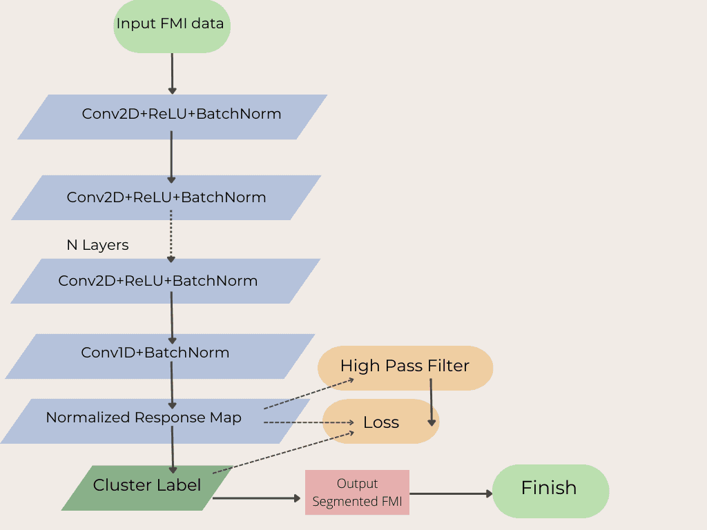
Unsupervised CNN segmentation architecture showing feature extraction, 1D conv to cluster space, batch norm, argmax labelling, and the two backpropagated losses — Unsupervised CNN segmentation pipeline — feature extractor → 1D conv to q=3 cluster space → batch norm → argmax labelling. Two losses (feature similarity + spatial continuity) backpropagate through the entire stack.

The full pipeline:

Input image → CNN feature-extraction module → deep features
1D convolutional layer projects features into a q-dimensional cluster space (we use q = 3)
Batch normalisation across the axes of the cluster space
Argmax assigns each pixel to its highest-scoring cluster ID
The cluster labels become pseudo-targets for the feature-similarity loss
Both losses backpropagate; the CNN learns to produce features that cluster cleanly and respect spatial continuity

Results — varying training duration and the spatial-continuity weight

We ran the network on real FMI sections at multiple operating points to understand its behaviour:

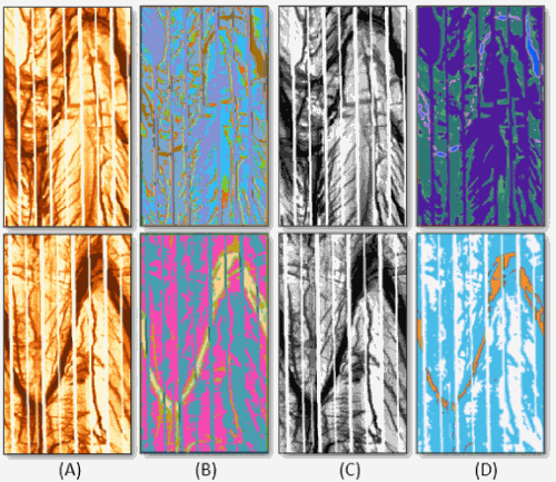
Cluster output animation showing 31 clusters at mu=0.1, 31 at mu=0.5, 20 at mu=1, 12 at mu=2, 19 at mu=3 — Effect of the spatial-continuity weight μ — higher μ collapses the segmentation toward fewer, larger clusters. μ ≈ 1 captures the bedding-plane structure cleanly; μ ≥ 2 over-smooths.

The cluster count varies non-monotonically with the continuity weight μ:

μ	Clusters detected (after 500 iterations)
0.1	31
0.5	31
1	20
2	12
3	19

Two takeaways:

μ ≈ 1 is the operating point for FMI logs. Below this, the segmentation over-fragments noise into spurious clusters. Above, it merges legitimate bedding planes.
The non-monotonicity at higher μ comes from the spatial-continuity loss interacting with the feature-similarity loss in non-trivial ways. Worth understanding before deploying this in a regulated workflow.

We also tested a scribble-guided variant — a hand-drawn scribble pre-seeds the cluster assignment in regions of interest:

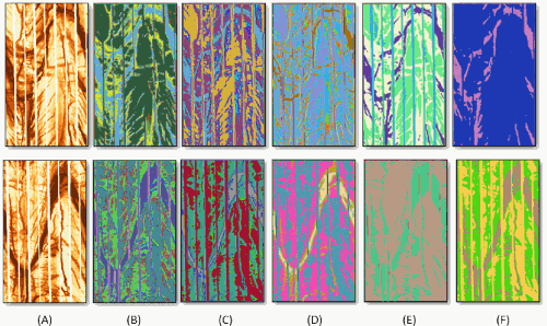
Scribble-guided segmentation showing 11 clusters identified after using a hand-drawn scribble — Scribble-guided segmentation — a hand-drawn scribble (panel C) pre-seeds the cluster assignment, giving the user a way to inject domain knowledge into the unsupervised pipeline.

This bridges the gap between fully-unsupervised (no labels at all) and fully-supervised (every pixel labelled). For production deployments, the scribble variant is the practical sweet spot — interpreters draw a scribble on a representative section, the network propagates that intent across the rest of the log.

The scribble-guided variant is the practical sweet spot — interpreters draw on representative sections, the network propagates the intent. Domain knowledge meets unsupervised learning at the right interface.

Conclusion

CNN-based unsupervised learning can identify the sinusoidal patterns of fractures and bedding planes in FMI logs without any labelled training data. The approach generalises cleanly across log vintages and basins where supervised models would need re-training.

Open question: how does the method behave on complex fractured regions — high-density fault networks where the linear-Hough assumption breaks down? That's the next study.

Reference

This work was presented at the EAGE Workshop on Borehole Geology in Asia Pacific (March 2021, Volume 2021, p. 1–7).

Key takeaways

Unsupervised CNN segmentation finds bedding planes and fracture sinusoids in FMI logs with zero labelled training data — the labelled-data bottleneck dissolves.
μ ≈ 1 is the operating point on FMI: below it the segmentation over-fragments noise; above it merges legitimate bedding planes.
Inter-interpreter disagreement on FMI fracture density is 20%+ for two senior geologists looking at the same log — automation isn't replacing accuracy, it's replacing variance.
The scribble-guided variant is the practical sweet spot for production deployments: interpreters draw on representative sections, the network propagates the intent.

Glossary

Breakout: An ovalised borehole cross-section caused by stress concentration at the wellbore wall. Visible on FMI as a pair of dark stripes 180° apart along the borehole axis. Predictive of wellbore-stability problems if not mitigated by mud-weight changes.
Canny edge detection: A multi-stage edge-detection algorithm (Canny, 1986) — Gaussian smoothing, gradient computation, non-maximum suppression, hysteresis thresholding. Produces clean single-pixel edges from noisy images. The standard preprocessing step before Hough transforms.
FMI: Formation Micro-Imaging — a borehole logging tool that produces a high-resolution micro-resistivity image of the wellbore wall. Reveals geological features (bedding planes, fractures, breakouts) at sub-centimetre resolution that conventional logs cannot.
GR: Gamma Ray log — measures natural radioactivity along the borehole. High readings indicate shales (more clay, more uranium/thorium); low readings indicate sands or carbonates. The default lithology indicator and depth correlator.
Hough transform: A feature-extraction technique that detects imperfect instances of geometric shapes (lines, circles, sinusoids) within a class via a voting procedure. Robust to noise and partial occlusion — the standard tool for extracting bedding-plane sinusoids from FMI images.
NPHI: Neutron Porosity log — bombards the formation with neutrons and measures the slowing rate, which depends on hydrogen content (water + hydrocarbons). The standard porosity proxy when run alongside density logs.
Otsu: Otsu's method (Otsu, 1979) — automatic image threshold selection that minimises intra-class variance. Produces clean binary images from grayscale inputs without requiring a manually-tuned threshold value.
Sonic: Sonic logging tools — measure the formation's compressional and shear-wave velocities. Used for porosity estimation, mechanical-property estimation, and (with seismic data) for time-depth conversion.
Unsupervised segmentation: Image-segmentation technique that requires no labelled training data. The network discovers segmentation structure from the image itself, typically by learning features that cluster coherently in feature space and respect spatial continuity.